Outline
History makes for good pedagogy with neural networks.
The simplest possible artificial neural network contains just one very simple artificial neuron – Frank Rosenblatt’s original perceptron.
(Rosenblatt’s perceptron is in turn based on McCulloch and Pitt’s even-more-simplified artificial neuron, but we’ll skip over that, since the perceptron permits a simple training algorithm.)
We’ll create an artifical neural network that consists of a single perceptron.
We’ll demonstrate that a single perceptron can “learn” basic logical functions such as AND, OR and NOT.
As a result, neural networks inherit the computational power of digital logic circuits: suddenly, anything you can do with a logical circuit, you could also do with a neural network.
Once we’ve defined the perceptron, we’ll recreate the algorithm used to train it, a sort of “Hello World” exercise for machine learning.
This algorithm will consume examples of inputs and ouptuts to the perceptron, and it will figure out how to reconfigure the perceptron to mimic those examples.
The limits of this single-perceptron approach show up when trying to learn the Boolean function XOR.
This limitation in turn motivates the development of full-fledged artificial neural networks.
And, that development has three key conceptual parts:
- arranging multiple perceptrons in layers to improve expressiveness;
- realizing that the simple perceptron learning algorithm is now problematic; and then
- graduating to full artificial neurons to “simplify” learning.
The full technical treatment of these developments is reserved for future articles, but you will leave this article with a technical understanding of the fundamental computational abstraction driving generative AI.
More resources
If, after reading this article, you’re looking for a more comprehensive treatment, I recommend Artificial Intelligence: A Modern Approach:

This has been the default text since I was an undergraduate, yet it’s received continuous updates throughout the years, which means it covers the full breadth of classical and modern approaches to AI.
What’s a (biological) neuron?
Before we get to perceptrons and artificial neurons, it’s worth acknowledging biological neurons as their inspiration.
Biological neurons are cells that serve as the basic building block of information processing in the brain and in the nervous system more broadly.
From a computational perspective, a neuron is a transducer: a neuron transforms input signals from upstream neurons into an output signal for downstream neurons.
More specifically, a neuron tries to determine whether or not to activate its output signal (to “fire”) based on the upstream signals.
Depending on where incoming signals meet up with the neuron, some are pro-activation (excitatory) and some are anti-activation (inhibitory).
So, without going into too much detail:
- A neuron receives input signals from upstream neurons.
- The neuron combines input pro- and anti-activation signals together.
- When net “pro-activation” signal exceeds a threshold, the neuron “fires.”
- Downstream neurons receive the signal, and they repeat this process.
What’s a perceptron?
The perceptron, first introduced by Frank Rosenblatt in 1958, is the simplest form of an artificial neuron.
Much like a biological neuron, a perceptron acts like a computational transducer combining multiple inputs to produce a single output.
In the context of modern machine larning, a perceptron is a classifier.
What’s a classifier?
A classifier categorizes an input data point into one of several predefined classes.
For example, a classifier could categorize an email as spam or not_spam.
Or, a classifier might categorize an image as dog, cat, bear or other.
If there are only two categories, it’s a binary classifier.
If there are more than two categories, it’s a multi-class classifier.
A single perceptron by itself is a binary classifier, and the raw output of a perceptron is 0 or 1.
Of course, you could write a classifier by hand.
Here’s a hand-written classifier that takes a single number and “classifies” it as nonnegative (returning 1) or negative (returning 0):
def is_nonnegative(n):
   if n >= 0:
      return 1
   else:
      return 0
Machine learning often boils down to using lots of example input-output pairs to “train” these classifiers, so that they don’t have to be programmed by hand.
For this very simple classifier, here’s a table of inputs and ouptuts:
Input:     5,    Classification: 1
Input:    10,    Classification: 1
Input:   2.5,    Classification: 1
Input:  0.01,    Classification: 1
Input:     0,    Classification: 1
Input:    -3,    Classification: 0
Input:  -7.8,    Classification: 0
Whether a given training algorithm can turn this into the “right” classifier – a close enough approximation of is_nonnegative – is a topic for a longer discussion.
But, that’s the idea – don’t code; train on data.
What’s a binary linear classifier?
More specifically, a perceptron can be thought of as a “binary linear classifier.”
The term linear has several related meanings in this context:
A linear classifier is a type of classifier that makes its predictions based on a linear combination of the input features.
And, for a linear classifier, the boundary separating the classes must be “linear” – it must be representable by a point (in one dimension), a straight line (in two dimensions), a plane (in three dimensions), or a hyperplane (in higher dimensions).
(All of this will make more sense once actual inputs are used.)
So, operationally, a perceptron treats an input as a vector of features (each represented by a number) and computes a weighted sum, before applying a step function to determine the output.
Because a perceptron classifies based on linear boundaries, classes that are not “linearly separable” can’t be modeled using just one perceptron.
Overcoming this limitation later motivates the development of full artificial neural networks.
The perceptron’s simplicity makes it an excellent starting point for understanding the mechanics of artificial neural networks.
The anatomy of a perceptron
An individual perceptron is defined by three elements:
- the number of inputs it takes, n;
- a list of of n weights, one for each input; and
- a threshold to determine whether it should fire based on the input.
The operation of a perceptron has two phases:
- multiplying the inputs by the weights and summing the results; and
- checking for activation:
- If the sum is greater than or equal to a threshold, the perceptron outputs 1.
- If the sum is less than the threshold, the perceptron outputs 0.
It’s straightforward to implement this in Python:
def perceptron(inputs, weights, threshold):
    weighted_sum = sum(x * w for x, w in zip(inputs, weights))
    return 1 if weighted_sum >= threshold else 0
And, then, we could re-implement is_nonnegative as a binary linear classifier:
def is_nonnegative(x):
    return perceptron([x], [1], 0)
Using this definition, we can also get a perceptron to simulate logical NOT:
def not_function(x):
    weight = -1
    threshold = -0.5
    return perceptron([x], [weight], threshold)

print("NOT(0):", not_function(0))  # Outputs: 1
print("NOT(1):", not_function(1))  # Outputs: 0
Learning: From examples to code
Tweaking weights by hand is an inefficient way to program perceptrons.
So, suppose now that instead of picking weights and thresholds by hand, we want to find the weights and threshold that correctly classify some example input-output data automatically.
That is, suppose we want to “train” a perceptron based on examples of inputs and desired outputs.
In particular, let’s take a look at the truth table for AND encoded as a list of input-output pairs:
and_data = [
 ((0, 0),  0),
 ((0, 1),  0),
 ((1, 0),  0),
 ((1, 1),  1)
]
Can we “train” a perceptron to act like this function?
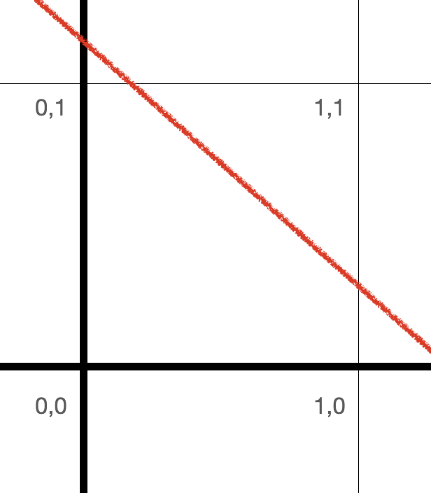
Because the input points that output 0 are linearly separable from the input
points that output 1, yes, we can!
Graphically, we can draw a line that separates (0,0), (0,1) and (1,0) from (1,1):
To find such a line automatically, we’ll implement the perceptron learning algorithm.
The perceptron learning algorithm
The perceptron learning algorithm is an iterative process that adjusts the weights and threshold of the perceptron based on how close it’s getting to the training data.
Here’s a high-level overview of the perceptron learning algorithm:
- Initialize the weights and threshold with random values.
- For each input-output pair in the training data:
- Compute the perceptron’s output using the current weights and threshold.
- Update the weights and threshold based on the difference between the desired output and the perceptron’s output – the error.
- Repeat steps 2 and 3 until the perceptron classifies all input-output pairs correctly, or a specified number of iterations have been completed.
The update rule for the weights and threshold is simple:
- If the perceptron’s output is correct, do not change the weights or threshold.
- If the perceptron’s output is too low, increase the weights and decrease the threshold.
- If the perceptron’s output is too high, decrease the weights and increase the threshold.
To update the weights and threshold, we use a learning rate, which is a small positive constant that determines the step size of the updates.
A smaller learning rate results in smaller updates and slower convergence, while a larger learning rate results in larger updates and potentially faster convergence, but also the risk of overshooting the optimal values.
For the sake of this implementation, let’s assume that the training data comes as a list of pairs: each pair is the input (a tuple of numbers) paired with its desired output (0 or 1).
Now, let’s implement the perceptron learning algorithm in Python:
import random

def train_perceptron(data, learning_rate=0.1, max_iter=1000):

    # max_iter is the maximum number of training cycles to attempt
    # until stopping, in case training never converges.

    # Find the number of inputs to the perceptron by looking at
    # the size of the first input tuple in the training data:
    first_pair = data[0]
    num_inputs = len(first_pair[0])

    # Initialize the vector of weights and the threshold:
    weights = [random.random() for _ in range(num_inputs)]
    threshold = random.random()

    # Try at most max_iter cycles of training:
    for _ in range(max_iter):

        # Track how many inputs were wrong this time:
        num_errors = 0

        # Loop over all the training examples:
        for inputs, desired_output in data:
            output = perceptron(inputs, weights, threshold)
            error = desired_output - output

            if error != 0:
                num_errors += 1
                for i in range(num_inputs):
                    weights[i] += learning_rate * error * inputs[i]
                threshold -= learning_rate * error

        if num_errors == 0:
            break

    return weights, threshold
Now, let’s train the perceptron on the and_data:
and_weights, and_threshold = train_perceptron(and_data)

print("Weights:", and_weights)
print("Threshold:", and_threshold)
This will output weights and threshold values that allow the perceptron to behave like the AND function.
The values may not be unique, as there could be multiple sets of weights and threshold values that result in the same classification.
So, if you train the perceptron twice, you may get different results.
To verify that the trained perceptron works as expected, we can test it on all possible inputs:
print(perceptron((0,0),and_weights,and_threshold)) # prints 0
print(perceptron((0,1),and_weights,and_threshold)) # prints 0
print(perceptron((1,0),and_weights,and_threshold)) # prints 0
print(perceptron((1,1),and_weights,and_threshold)) # prints 1
Learning the OR Function
Now that we’ve successfully trained the perceptron for the AND function, let’s do the same for the OR function. We’ll start by encoding the truth table for OR as input-output pairs:
or_data = [
    ((0, 0), 0),
    ((0, 1), 1),
    ((1, 0), 1),
    ((1, 1), 1)
]
Just like with the AND function, the data points for the OR function are also linearly separable, which means that a single perceptron should be able to learn this function.
Let’s train the perceptron on the or_data:
or_weights, or_threshold = train_perceptron(or_data)

print("Weights:", or_weights)
print("Threshold:", or_threshold)
This will output weights and threshold values that allow the perceptron to behave like the OR function. As before, the values may not be unique, and there could be multiple sets of weights and threshold values that result in the same classification.
Once again, we can test it on all possible inputs:
print(perceptron((0,0),or_weights,or_threshold)) # prints 0
print(perceptron((0,1),or_weights,or_threshold)) # prints 1
print(perceptron((1,0),or_weights,or_threshold)) # prints 1
print(perceptron((1,1),or_weights,or_threshold)) # prints 1
Limits of a single perceptron: XOR
Having trained the perceptron for the AND and OR functions, let’s attempt to train it for the XOR function.
The XOR function returns true if exactly one of its inputs is true, and false otherwise. First, we’ll encode the truth table for XOR as input-output pairs:
xor_data = [
    ((0, 0), 0),
    ((0, 1), 1),
    ((1, 0), 1),
    ((1, 1), 0)
]
Now let’s try to train the perceptron on the xor_data:
xor_weights, xor_threshold = train_perceptron(xor_data, max_iter=10000)

print("Weights:", xor_weights)
print("Threshold:", xor_threshold)
For my run, I got:
Weights: [-0.19425288088361953, -0.07246046028471387]
Threshold: -0.09448636811679267
Despite increasing the maximum number of iterations to 10,000, we will find that the perceptron is unable to learn the XOR function:
print(perceptron((0,0),xor_weights,xor_threshold)) # prints 0
print(perceptron((0,1),xor_weights,xor_threshold)) # prints 1
print(perceptron((1,0),xor_weights,xor_threshold)) # prints 1
print(perceptron((1,1),xor_weights,xor_threshold)) # prints 1!!
The reason for this failure is that the XOR function is not linearly separable.
Visually, this means that there is no straight line that can separate the points (0,1) and (1,0) from (0,0) and (1,1).
Try it yourself: draw a square, and then see if you can draw a single line that separates the upper left and lower right corners away from the other two.
In other words, because perceptrons are binary linear classifiers, a single perceptron is incapable of learning the XOR function.
From a perceptron to full artificial neural nets
In the previous sections, we demonstrated how a single perceptron could learn basic Boolean functions like AND, OR and NOT.
However, we also showed that a single perceptron is limited when it comes to non-linearly separable functions, like the XOR function.
To overcome these limitations and tackle more complex problems, researchers developed modern artificial neural networks (ANNs).
In this section, we will briefly discuss the key changes to the perceptron model and the learning algorithm that enable the transition to ANNs.
Multilayer Perceptron Networks
The first major change is the introduction of multiple layers of perceptrons, also known as Multilayer Perceptron (MLP) networks. MLP networks consist of an input layer, one or more hidden layers, and an output layer.
Each layer contains multiple perceptrons (also referred to as neurons or nodes). The input layer receives the input data, and the output layer produces the final result or classification.
In an MLP network, the output of a neuron in one layer becomes the input for the neurons in the next layer. The layers between the input and output layers are called hidden layers, as they do not directly interact with the input data or the final output.
By adding hidden layers, MLP networks can model more complex, non-linear relationships between inputs and outputs, effectively overcoming the limitations of single perceptrons.
Activation Functions
While the original perceptron model used a simple step function as the activation function, modern ANNs use different activation functions that allow for better learning capabilities and improved modeling of complex relationships.
Some popular activation functions include the sigmoid function, hyperbolic tangent (tanh) function, and Rectified Linear Unit (ReLU) function.
These activation functions introduce non-linearity to the neural network, which enables the network to learn and approximate non-linear functions.
In addition, they provide “differentiability” (in the sense of calculus), a critical property for training neural networks using gradient-based optimization algorithms.
Backpropagation and gradient descent
The perceptron learning algorithm is insufficient for training MLP networks, as it is a simple update rule designed for single-layer networks.
Instead, modern ANNs use the backpropagation algorithm in conjunction with gradient descent or its variants for training.
Backpropagation is an efficient method for computing the gradient of the error with respect to each weight in the network. The gradient indicates the direction and magnitude of the change in the weights needed to minimize the error.
Backpropagation works by calculating the error at the output layer and then propagating the error backward through the network, updating the weights in each layer along the way.
Gradient descent is an optimization algorithm that uses the computed gradients to update the weights and biases of the network. It adjusts the weights and biases iteratively, taking small steps in the direction of the negative gradient, aiming to minimize the error function.
Variants of gradient descent, like stochastic gradient descent (SGD) and mini-batch gradient descent, improve the convergence speed and stability of the learning process.
Onward
In short, the transition from single perceptrons to full artificial neural networks involves three key changes:
- Arranging multiple perceptrons in layers to improve expressiveness and model non-linear relationships.
- Introducing different activation functions that provide non-linearity and differentiability.
- Implementing the backpropagation algorithm and gradient descent for efficient and effective learning in multilayer networks.
With these changes, ANNs become capable of learning complex, non-linear functions and solving a wide range of problems, ultimately leading to the development of the powerful generative AI models we see today.
Future articles will delve deeper into each of these topics, exploring their theoretical foundations and practical implementations.
Further reading
Michael Nielsen has an excellent free online textbook on machine learning that also begins with perceptrons.
Stephen Wolfram wrote a long and highly detailed explanation of machine learning all the way up through the technical development of ChatGPT.
The textbook Artificial Intelligence: A Modern Approach by Russell and Norvig cover the full breadth of AI from classical to modern approaches in great detail:
Twitter: @mattmight
Instagram: @mattmight
LinkedIn: matthewmight
Mastodon: @mattmight@mathstodon.xyz
Sub-reddit: /r/mattmight